Now that there’s only 3 semesters left of my university career, we wanted to try something new. I have never worked with radio systems much and particularly not radar. Thus when the oppertunity to do a project within Numerical Scientific Computing, my prosective group member and I went to one of the professors in the communications department and asked if he had a project that we could work on. He suggested we could work on a target tracking radar system utilizing a track-before-detect (TBD) algorithm. He actually presented a paper that he had cowritten showcasing a radar signal model, target state-space model and an algorith called a Particle Filter. Needless to say, we accepted his proposal and started researching. The goal of the project would be to create a simulation model that could be used to evaluate the computational complexity of such a tracking system.
Since we knew absolutely nothing about radar systems we took to the internet and some recommended books from our supervisor. Ofcourse we commited the usual crime of throwing ourselves over the actual algorithm before we had gotten an overview of what different kinds of radar systems was available. However we know that we wanted to see if we could simulate a Multiple-Input Multiple-Output (MIMO) system using the signal model from the article our supervisor had cowritten, by the way, the article can be found here.
So let’s see what kind of usecase we can create for this radar system.
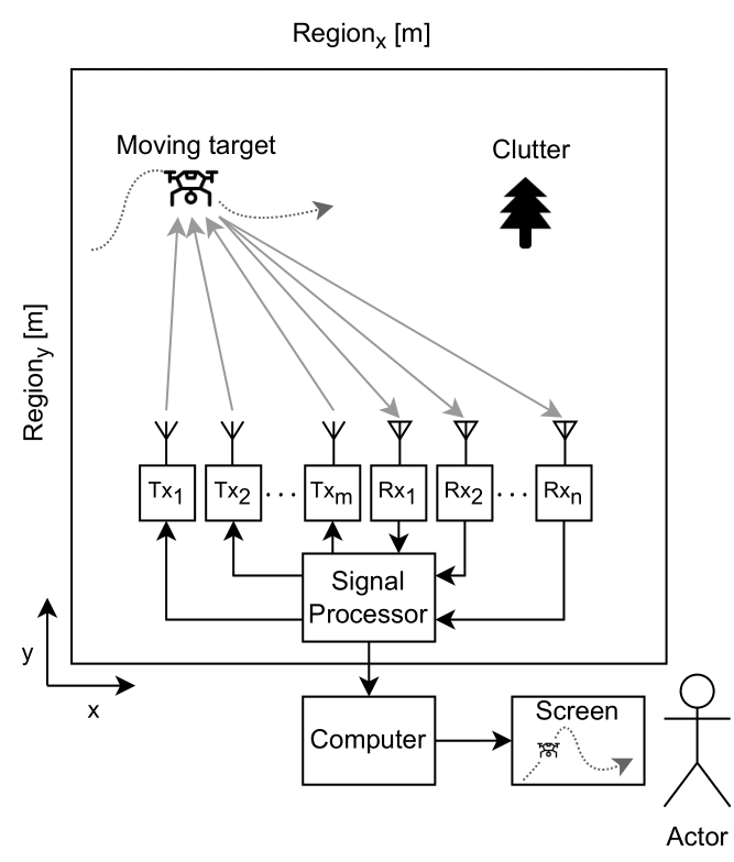
We want to have an array of transmitter antennas and receiver antennas. The transmitters will send out a signal that will bounce of any present targets, but also other objects which we will call clutter. Since we don’t have any actual antennas, we need to simulate how a signal would propagate from one antenna, to a target, to another antenna. How should the antennas even be placed in relation to each other? (Note: we will not be taking full use of the advantages that a MIMO system brings to the table because of the limited amount of time a semester offers.)
Next, any radar system needs a signal processing box, because otherwise we would just be receiving weird samples from an antenna. So our code will be focused mostly around this signal processing box.
After the signal processing box we need to use some hardware that contains some more power for the heavy lifting. By that I mean the estimation algorithm. Since we have chosen to implement a particle filter, the same calculations must be run when updating each particle in each observation.
Radars
Okay, let’s first talk a little bit about how radars actually work before diving deeper into the topic of implementing and testing the algorithms. Radar is an old acronym for RAdio Detection And Ranging. Meaning we use electromagnetic radio signals to determine if there is something out there, and in the case there is, how far away it is from the observation point. When emitting a radio wave it will travel in different direction depending on the gain and directivity of the transmitting antenna and (hoepfully) reach an object.
Types of Radars
Generally we talk about two types of radar systems that is, monostatic and multistatic systems. In a monostatic system, the receiver and transmitter in build into the same radar hardware. Meaning that only one antenna is used for both transmitting and receiving. Within those systems there are again several different way to create a signal for transmission. Some of the modulation types will be discussed later.
In multistatic systems, the receiver and transmitter are two seperate parts of hardware with their own associated antennas. When talking multistatic systems, there are several different termonoligies that describes how the receivers and transmitters are physically placed in relation to each other. They can be colocated meaning, they are closely spaced. In traditional radars, this usually refers to a monostatic radar. However in MIMO radar we can have colocated antennas without the being monostatic. In fact, colocated MIMO is often used because it is possible to create a virtual antenna array, which makes it possible to run some interesting beamforming algorithms.
The idea of this project was to look at the system in a multistatic MIMO setup, which we technically did. We ended up spending so much time on the actual implementation of the basic radar system that we did not consider much of the benefits that MIMO brings to the table such as beamforming and virtual arrays. Which is a bummer because this is one of the research areas within radar that still has a lot of uncovered grounds.
The Radar Equation
Depending of the Radar Cross Sectional (RCS) area of the object, some energy will be reflected back toward our receiver. The RCS can be a very tricky thing to calculate and it depends on a lot of things. For bladed aircrafts such as commercial drones, it can even depend on the position of the rotors. The military uses special paint on their stealth aircrafts in order to lower the RCS. The recieved power from a reflected wave can be expressed by the radar range equation as shown below
$$P_r = \frac{P_t G_t G_r \lambda^2 \sigma}{(4\pi)^2 R^4 L_a(R)}$$
Where $P_t$ is the transmitted power, $G_t, G_r$ is gains of the transmitter and receiver, $\lambda$ is the wavelength of the carrier, $\sigma$ is the RCS, $R$ is the distance and $L_a(R)$ is an attenuation factor determine by wavelength, media and altitude. This factor can be read of a figure in many rader theory books such as Fundamentals of Radar Signal Processing by Mark A Richards - I would recommend this books to anyone interested in learning more about radar theory and the signal processing aspect.
For the RCS we found a figure of some common DJI commercial drones in a NATO paper - Drone RCS Statistical Behaviour.
So we can quickly see from the equation that the received signal strength will decrease very rapidly the further the target is from the observation point. In our implementation we’ve assumed, so far, that antennas are isotropic (even the they are wildly directional) and that the gains are optimal at $1$. Thus we can use the to determine the maximum distance that we can detect and track a target from
$$R_{max} = \sqrt[4]{\dfrac{P_t G_t G_r \lambda^2 \sigma}{(4\pi)^3 S_{min} L_a(R)}}$$
Where $S_{min}$ is the minimum detectable signal power before the signal is just lost in noise in the receiver. There are also influence from the earths surface and curvature that can be implemented into the mathematical model. For example the signal can hit the ground and be reflected from there onto the target and back to the receiver. This would increase the observed delay between transmission and reception. However we have not considered that for this project. Which means that $S_{min}$ will be defined by the SNR in the receiver.
Radar Modulation
So in order to actually use the theories we just discussed in relation to the radar equation in practice, we first need to send out a signal. The modulation could either be a continous wave (CW) waveform were we either use no modulation, use frequency modulation, or phase modulation. The other way we can go is to send out a series of pulses, basically turning the transmitter on and of, usually very fast. Here we can either stick with the pure pulse, or we can start using modulation inside the pulse. As with CW we can use frequency or phase modulation. For ranging and angle estimation purposes, we often use a Frequnecy modulated Continous Wave Radar (FMCW). The name can be a little devious, because what we are acuatlly doing is sending out a series of pulses with frequency modulation. The total series of pulses is called a frame.
An FMCW radar will over a period of a pulse, linearly change the frequency of the signal from $f_{min}$ to $f_{max}$. When receiving the signal after it having bounced of the target, we will use a mixer in order to mix the original signal with the time delayed received signal. This is shown in the image below.
The FMCW Radar uses a Fourier Transform on the received signal in order to determine
Using FMCW Radar, we only need a single transciever in order to determine the range of our target, provided the target being in range. If however, we want to get some velocity and angle information about our target, this is also possible using FMCW. The idea of the pulse train come in when we start looking at the velocity of the target. Because a moving target will cause a very small change in doppler frequency when the wave is returned. This change is not enough for us to distinguish between velocities. However the phase will have a quite significant change associated with it. Therefore, we can exploit the change in phase between pulses and thus estimate the velocity with pretty good accuracy.