The first semester of the master studies in Signal Processing was more or less an introduction to signal processing within audio systems. We had a few project proposals from external companies. My project group and I (4 people in total), found a few of the proposals from the company RTX A/S interesting. RTX works a lot in the audio domain and develops a great deal of headset technology. They were interested in some student investigating more into classification of acoustic scenes using neural networks. They did not provide us with a whole lot of information as to what they could use such a technology for, however we discussed that a great use case would be some adaptive noise cancellation algorithms.
The 1st semester of the masters degrees at our institute is also where we are required to write a scientific paper around our project. A conference called SEMCON is then held at the end of the semester. This is a great way to have a gentle introduction into the whole aspect of scientific methods and writing. The paper had to be 6 pages and since it was a conference, we were also required to make a poster. Although the physical conference was cancelled due to Covid-19, it was still a valuable insight into the academic/scientific community.
So we had chosen our project and then had to narrow down to a case that we wanted to work with. That is, we had to choose a well defined area with different acoustic scenes to try to classify. After a lot of consideration, we ended up going with a construction site. Here we saw four obvious acoustic scenes: Inside, outside, office and inside a vehicle. We also ended up defining a fifth scene: semi-outside, however as the results will show, this was either badly defined or our training data was not good enough. We got in touch with the company overseeing the construction of NAU (Nyt Aalborg Universitetshospital), which is a huge construction site of the new university hospital in Aalborg. They agreed to let us come by with some recording equipment and get some data for our classifier. This yielded around 2-3 hours of recordings. Below is an image of one the recording setups at NAU.
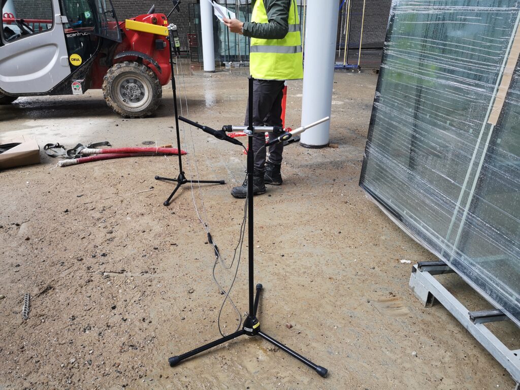
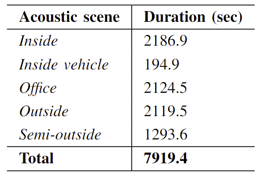
As the image shows, we used a handy-recorder with two internal microphones and two external microphones that had good omni-directional properties. This meant that we ended up with the duration of recordings as shown in the table below.
Having some initial data to run some tests on, we set out to some preprocessing in order to use the data as an input to a neural network. For the network architecture we chose to go with a Convolutional Neural Network (CNN) as previous work had shown this structure to be very successful in acoustic scene classification. More specifically we chose to go with a 2D CNN. Meaning inputs should be 2D arrays. Usually one would use images as inputs for such a network structure. Which is why we chose to convert our data into spectrogram representations. This way we could also ensure a somewhat data-driven approach to training the network. Although some would probably argue that the complete data-driven approach would be to train on the raw waveform data.
Anyway, by converting the images into spectrograms it meant that we could keep the opportunity to add noise to the data in the time domain before conversion into the time-frequency domain. We utilized this when doing the actual robustness testing of the network. This was also the core part of the actual study regulations for the semester together with the recordings. The conversion to spectrograms and saving as images also gave us some data augmentation as the images were saved as RGB. So we went from time series data to 3-dimensional time-frequency data. Neural networks was not a part of this semester’s description and was therefore an added bonus (more work). So our preprocessing module ended up having the flow as shown below
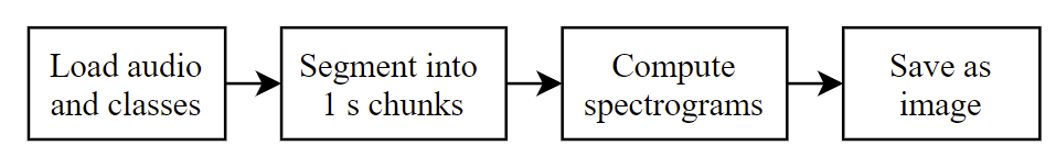
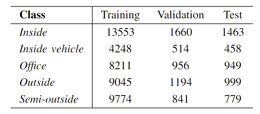
Saved images where then split into three different categories: training, validation and test. Since the neural network was implemented using the Python Keras library, this is the structure that was expected for training the network. We used an 80%, 10%, 9% distribution, so that we got the following amount of images.
As the figure shows the audio data was separated into 1 second chunks and the spectrograms where then computed using 1024 for the FFT size with an overlap of 512. The sample frequency used for collecting the data was 44.1 kHz.
We then designed a very very simple CNN architecture using Keras with two convolutional layers, two max pooling layers, a flattening layer and a dense (output) layer. The structure can be seen in the figure below
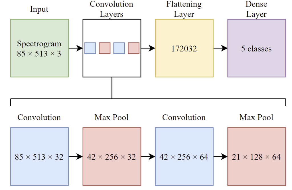
Kernel sizes for the convolutional layers and the max pooling layers were more or less arbitrarily chosen as most recommendation online seemed to suggest these sizes.
One of the core issues with using images as representation for audio data (specifically for acoustic scene classification) is that acoustic scenes are not very static. For example, if we take a look at our outside class, then at one point in time a drill or hammer go on in the background or a vehicle might drive by. This will change the spectrogram image quite a bit. Actually so much that a human would most likely not be able to tell that it is from the same class. If you take a classic example of the use case of a CNN, it would be to do image classification i.e. being able to determine that the image of a car is actually a car. The difference between the classic example and our example though, is that if you go out of your house and take a picture with your phone of your car. Then you wait 5 minutes and take the image again. The car will look exactly the same in those two images. There might be some differences in noise around the car, but the actual object you are trying to classify will look the same. However if you do an audio recording in exact some spot twice, 5 minutes apart, you might end up with completely different results for the image spectrograms. Which means we have this limitation in the system that we have to be aware of. To be honest, in order to somewhat overcome this, one would probably need a lot more training data than what we had.
With that out of the way, we started testing the network and the initial results showed between 90-98% accuracy. So instead of working more on the network structure, we started to add some noise into the testing data, so that we could see if and how much the accuracy would drop in different noisy conditions.
RTX had given us a potential use-case, where audio would be picked up by a headset, then sent to a base station where preprocessing and CNN classification would be made. Then results are sent back to the headset that can then be used for adaptive noise cancellation.
Considering this, we wanted to try to emulate a very very very simple simulation of a wireless communication channel. And when I say simple, I mean that the only thing we want to actually simulate, is some sort of gaussian noise process and some packet loss. The latter being the main concern expressed by RTX in their communication links. In order to do the packet loss, we had to collect the data into packets. We chose to use a packet size of 10ms (recommendation from RTX). Noise was then added according to the figure below
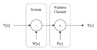
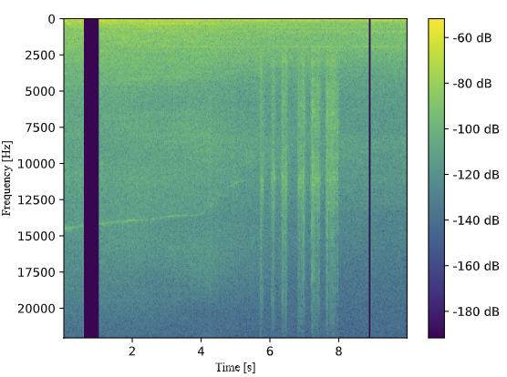
Where n was defined to be an entire packet and not just one sample. The system block would add white gaussian noise and the wireless channel with P[n] would introduce packet loss in either bursts or randomly with a certain probability. The figure below shows a spectrogram with added white gaussian noise and packet loss in bursts
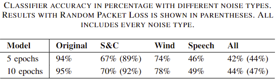
We also tried adding wind and speech onto the signal in order to simulate real world conditions more closely. Though wind noise is not an additive noise type, it seemed to have similar properties on the playback as the recorded wind. Overall our results can be seen in the table below.
If you would like to read our paper, you can download it and our conference poster can be downloaded here.