My 6th’s semester was writing my bachelor thesis. I worked on a project for the thesis with 3 of my fellow students. I have a Creality Ender 3 3D printer at home that I use for my hobby projects. I had seen a few projects trying to use deep learning to give people a heads up whether their print was failing.
However the current methods would only tell you if the printer started making “spaghetti”. Since we were working on a thesis in Vision Graphics and Interactive Systems, I proposed to my group that we could do a project around detecting errors in 3D prints. They ended up thinking it was a good idea as well. We pitched the idea to our supervisor and he liked it as well.
So we started laying out the system, we knew we had Octoprint on a Raspberry Pi 3b+ that was used as a web UI to control the printer. It was then pretty natural to use Octoprint in the project, because many hobbyist uses it to control their printers. Meaning we now had the first physical part of the system described.
We still needed something that we could actually analyze. Octoprint has an image capturing feature, but if we wanted to use that, we needed a camera.
We wanted to go with a low cost camera solution, mainly for two reasons. First, we wanted to see if a cheap camera would have high enough resolution to actually reveal errors in the prints. Secondly, we wanted a potential implementation to be cheap enough for hobbyists to use.
We could have easily just borrow a 5,000 USD camera from the university. But where’s the fun in that? And if your camera is more expensive than your printer, something’s wrong. We ended up making a table of the cameras we had readily available (it was Corona times after all and we couldn’t wait too long to get a camera in hand). The table is shown below.
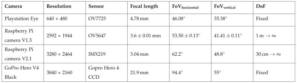
We required the camera to have a resolution that, at the distance given to the build platform, would give us at least 1 pixel per layer. I will explain later why we thought this was a good idea. We also required the camera to give us a pixel density at a given distance of 0.2 mm or better.
This is because 0.2 mm is the most commonly used layer height for FDM hobby 3D printers. We also needed the camera to be very fast in taking the pictures. The reason for this being that it is much easier to do image manipulation with the actual print only. Meaning we wanted to move the print head out of the frame for each photo. This was already implement in some of the Octoprint extensions for creating a timelapse of your print without having the printhead in the way.
Buuuuut…. When moving the printhead and leaving it in a position away from the model for an extended period of time you start to get what is called “oozing”. This is where the material inside the print nozzle starts to slowly make its way out of the nozzle head, due to the high pressure inside the nozzle. When the printhead then moves back to the print, the oozed material will then show up as artifacts on the surface of the print. Which in turn would be an error in the model. So we would basically end up potentially classifying errors that we had made ourselves.
System Definition and First Steps
The camera selection process itself wasn’t very scientific and we ended up using a Raspberry Pi V2 camera, as it is widely available and frequently used in the 3D printing community. This meant we could setup our system diagram to look like this
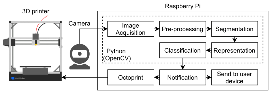
So as seen in the diagram, pretty all of the implementation was to be made on the Raspberry Pi. We had had a course in Image Processing, we wanted to use some of the theory from that to create a preprocessing and segmentation module. During the course we had also had some theory around machine learning algorithms.
We wanted to compare classification with some of those algorithms, to a simple feature threshold classification. We never made it to the notification part of the system, but we thought it was important to show our thought process in the diagram.
The camera setup was pretty simple. We calculated the distance the camera had to sit from the printers build plate in order to capture the full print volume. We then 3D printed and arm that extended from the printers base, and mounted the camera and Raspberry Pi onto it.
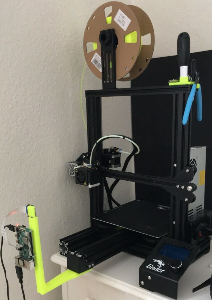
In order to put some limitations on the project, we hung up black card board behind the printer. This made it so that all of the images had a black background and thereby easier to process. Changing backgrounds could most likely be accounted for with some more software, however we did not want to focus on this.
The next problem we had to tackle, was how to find the actual print in the images. We knew what the model had to look like (in theory) since we had the 3D CAD model of the print. However there are slight differences between the 3D CAD model and the model that has gone through slicer software in order to be printed.
Instead of using the CAD model, we wanted to represent the model using the sliced GCODE. An FDM 3D printer prints a model in layers, therefore we have to do the so-called “slicing” in order to slice the model into printable layers. The output of this process is a GCODE file which contains a set of machine commands that is sent to and interpreted by the 3D printer’s firmware.
We can use this GCODE file to do a 3D plot in Python. An example of this can be seen in the figure below
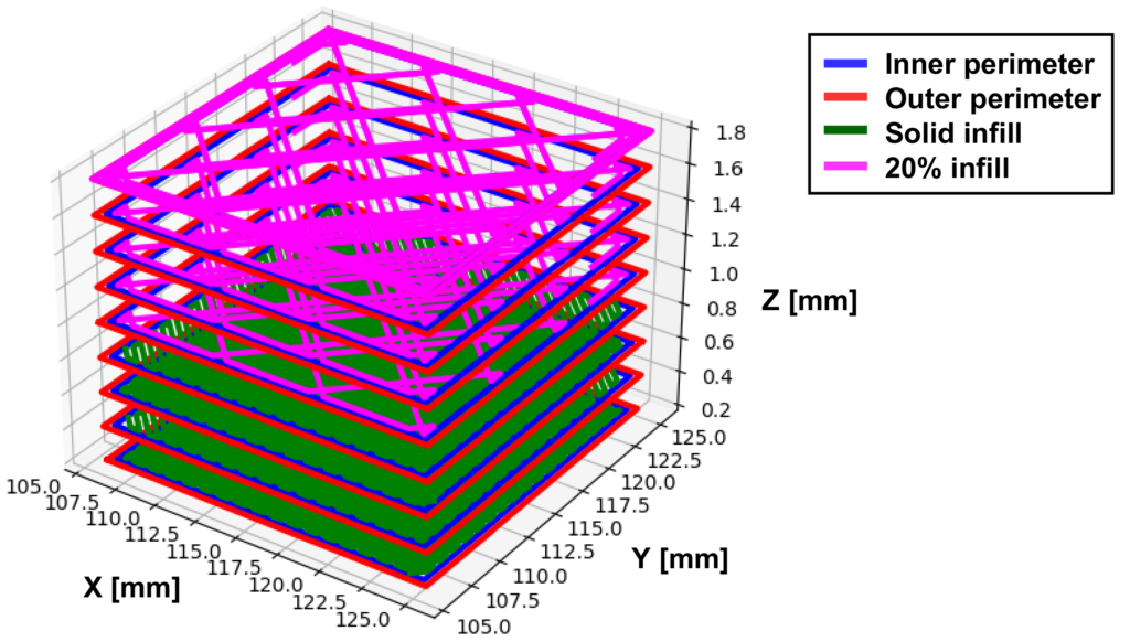
It is basically just a matter of plotting all the movement commands from the GCODE file and then adding the layer height to the z-value every time there is a layer change. The different colors represents the different parts of the layer printing procedure, i.e. the green color is solid infill, the red is outer perimeters, blue is inner perimeters and pink is non-solid infill.
We seemed to have an issue with the fact that there were no z-height on the plotted (simulated) models. However on all of the models that we used, there were enough layers for it to not matter. So we ended up just going with it.
So the next thing we wanted to do before developing too much of the algorithm, was to define which print issues we should detect. There are many things that can go wrong in a print, but we wanted to be able to determine the ones that would be most catastrophic. So we came up with the following table
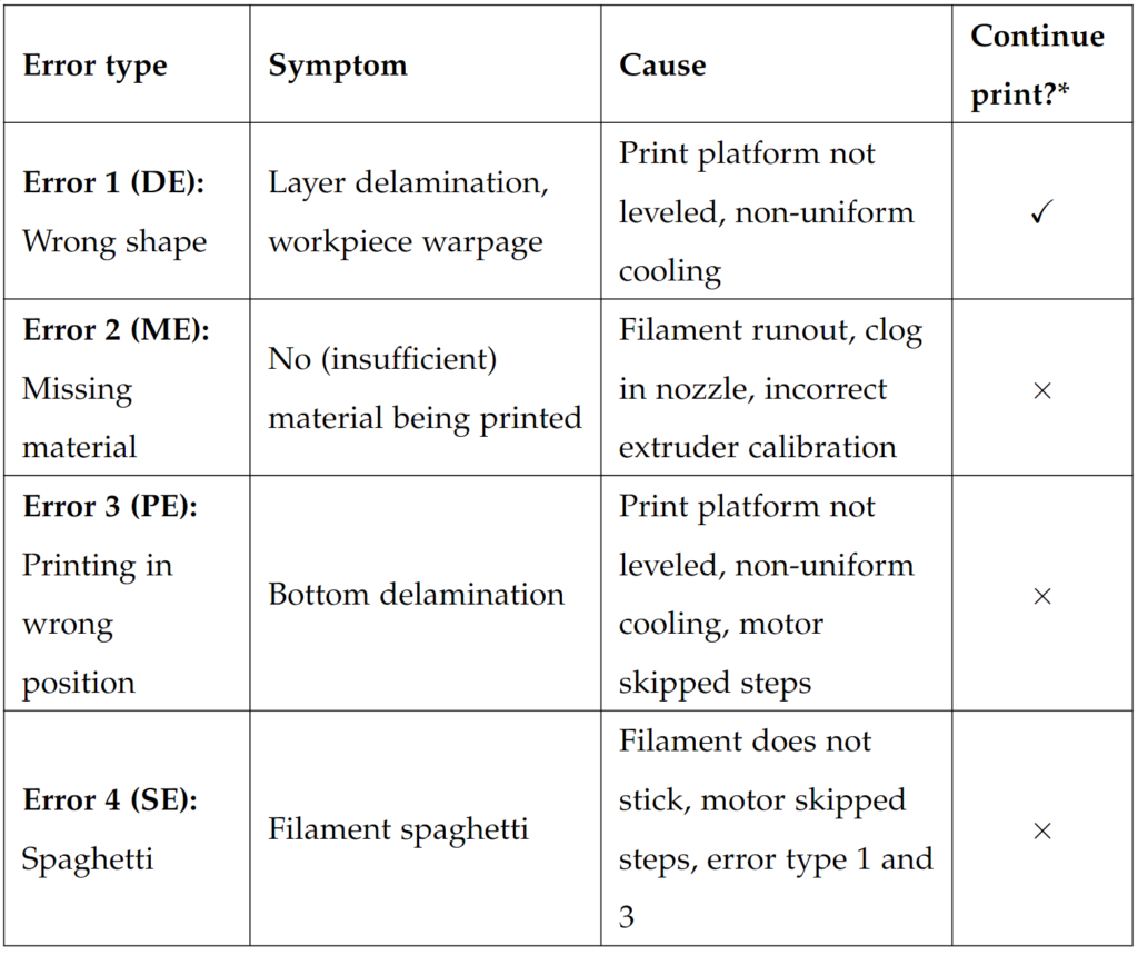
According to the table above, what we would be looking for in our vision algorithm was the symptoms of an error. In some cases we would then be able to make an educated guess on what the cause was. The only error where we would allow the print to continue was the layer delamination error, which inherently also was the one we expected to have the most trouble classifying.
At this stage of the project, we also did some research into what other implementations of vision algorithms where already out there for this purpose. What we found was that none of the existing systems were able to detect all of the above errors by itself. It would require an ensemble of all the current solutions to detect all error types.
Next thing we did was then to start implementing (well actually we made a requirements specification for the system first but I won’t bore you with the details of that). As I described earlier, we needed to move the printhead out of the way before we could capture an image, so that was one of the first things we started working on.
To do this, we used an OctoPrint plugin called GCODE System Commands, which is pretty awesome. Basically it let’s you create your own custom GCODES, that when read by OctoPrint, is able to execute system commands on the Raspberry Pi Linux system. All we needed to do was to just write a small shell script that we execute the commands to take the picture and save it to the desired location. Then we could use the plugin execute the script.
Before uploading the GCODE file to OctoPrint for printing, we wrote a Python script that would inject our custom code to move the printhead back/forth and take the picture.
| |
Since we could now make a model in 3D that we could use for comparison and we could inject custom GCODE, we were ready to start developing the image processing chain. First thing we started to tackle was the segmentation.
Image Processing Chain
I previously described that we wanted to use convolution to match our rendered 3D model of the GCODE to the actual print on the platform. A procedure known as template matching in the image processing world. This was done as shown in the image below
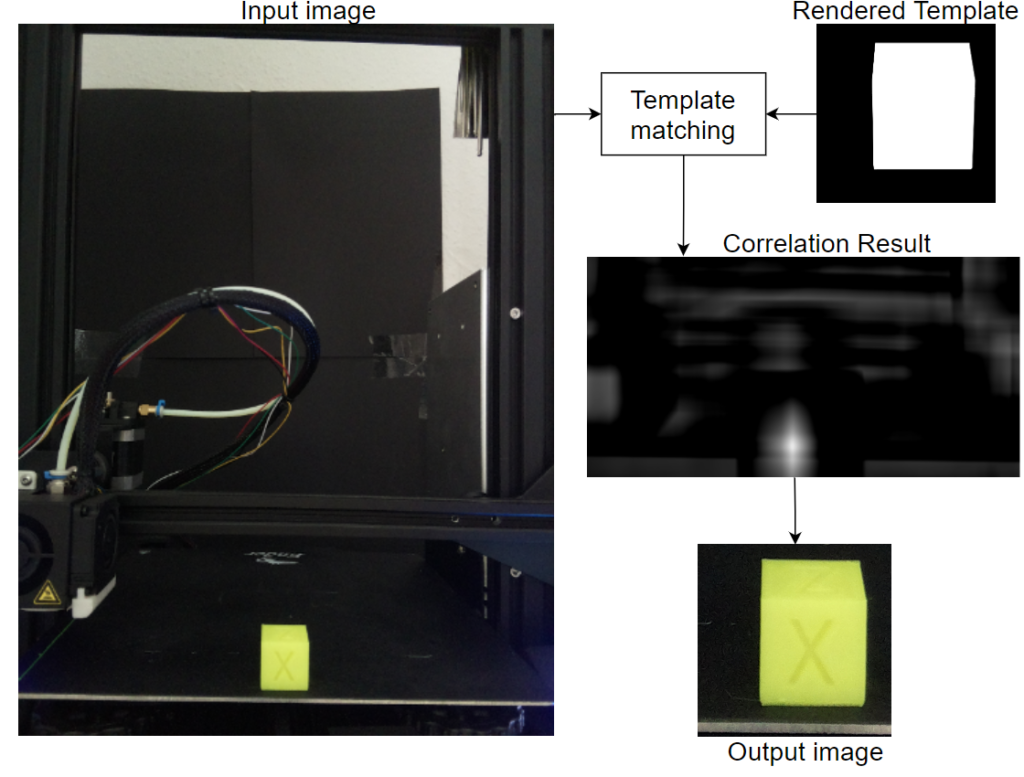
We would refer to the model as the template here. The template matching procedure outputs a map of correlation coefficients. The highest correlation between the template and the image, will be the brightest pixels on the correlation result above. The output image is then taken from the area with the highest correlation and will be the same size as the template.
Since the printing was done using a single color bright filament, we were able to use a simple threshold based on HSV to distinguish the background from the object of interest. This is definitely not ideal when using a material, that has a color closer to the print platform color.
It would also present issues when the print get’s tall enough such that the background is captured as well. Since we used black cardboard for the background it did not show up as an issue in our implementation. However for a more practical system, this would need to be accounted for.
Having done the segmentation of the captures images, we turned our attention to feature extraction. In our course we had been taught about some well known features that we could look for in shapes. These are features such as: area, circularity, perimeter, width, height, etc.
Features were extracted from both the rendered model and the captured images. In this way, we were able to actually compare the features between the two. What we did next, was to create a score vector.
We created the score vector my taking the minimum score between the rendered and captured image features and dividing it by the maximum between the two. Thereby normalizing the score vector. We then used three different models to evaluate whether our score vectors we a good method. Results can be seen in the image below
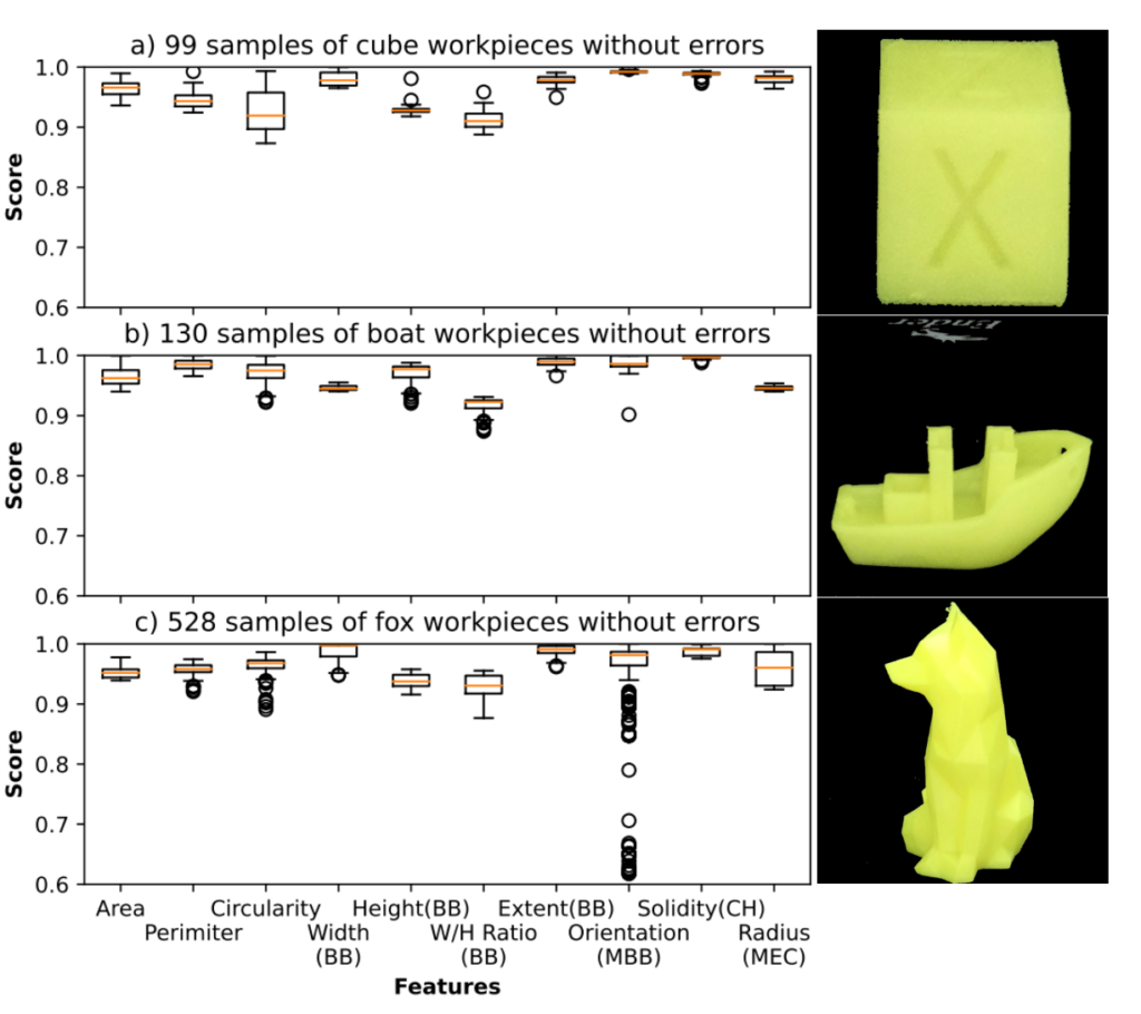
We used this method to get rid of some features that did not convey good information as well. For example, the orientation feature had a lot of deviation for the median in the fox model. So that suggested to us, that the feature becomes more unreliable as the number of layer get larger.
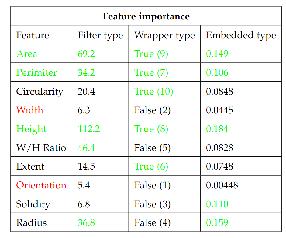
Different methods suggested that we should investigate the feature importance of each feature. This was done using the SciKit-learn feature selection toolbox in Python. The result can be seen in the image below.
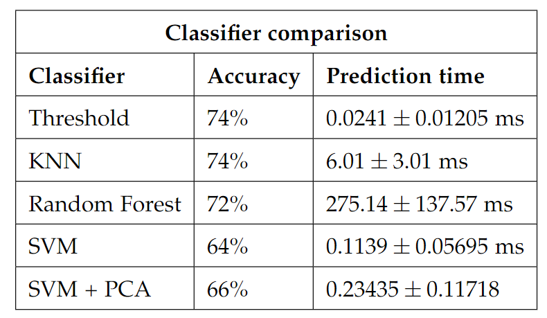
For the classification part of the system, we tried some different methods. As mentioned previously, we wanted to compare a threshold method to some of the well know Machine Learning algorithms such as k-nearest neighbors, Random Forest and Support Vector Machine.
Our results showed that the threshold method and k-nearest neighbors actually performed best and even equally well as shown below.
I hope you got something out of this. If you feel like I missed something, please let me know in the comments and I’ll try to elaborate.