Bode Plots in Python

This notebook will go through a pratical example of how to do bode plots in Python and how to find several other control related charateristics. We’ll look at an actual transfer function and derive all the information from that.

Let’s start off by importing the Python libraries that we are going to need. If you are not able to import the library, please install it using pip in your terminal or command prompt.

import matplotlib.pyplot as plt
import matplotlib
import control
from scipy import signal
from control import tf

%matplotlib inline
matplotlib.rcParams['figure.facecolor'] = 'w'

Now let’s define the transfer function that we are going to look at. We’ll look at an open loop transfer function from a mechanical system that is regulated. The method will work for transfer function in mechanics and electronics though

$$OL(s)=20\cdot \frac{300}{(0,01s+1)(0,1s+1)}\cdot 0,0033$$

Now to actually use the python libraries, we want the transfer function to be on a different form. The form should be $s^2+s+k$. So we’ll make sure to dissolve the parantheses in the denominator

$$OL(s)=20\cdot \frac{300}{0,001s^2+0,011s+1}\cdot 0,0033$$

Now that we have the expression in the correct form, we can put it into our first Python function. The function comes from the classsignal from the scipy library. We imported it just before by saying from scipy import signal. Now we are going to use a method from that class called lti. lti takes in several parameters, but we are only going to use two of them in this example. The first parameter is the numerator of our transfer function. The input should be in brackets [] and we are going to multiply everything together. So the first input would be [20*300*0.0033].

The second input will be the denominator of our transfer function. So we have $0,001s^2+0,11+1$. If we remove the $s$’s we get the second parameter which would then be [0.001, 0.11, 1]. As you can see we seperate the values by a comma.

Now let’s put all of this into our class method and assign it to the variable system

system = signal.lti([20*300*0.0033], [0.001, 0.11, 1])

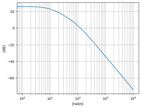
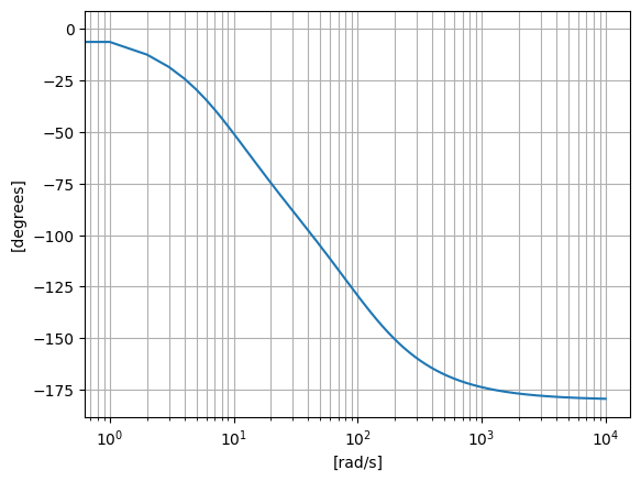
Now the signal.lti doesn’t do much for us. We want to have a bode plot, so we’ll have to use yet another method from the signal class to create the bode plot. The method signal.bode will do the trick. This returns three things: a frequency array in rad/s, a magnitude array in dB, and a phase array in degrees.

So when we call this method we want to assign in to three different variables. The first return value will be the frequency array and we’ll assign that to the variable w. The next return value will be the magnitude array and we’ll assign that to the variable mag. The last return value will be the phase array and we’ll assign that to the variable phase.

We’ll also need to tell the program the range of frequencies we want to look at (this is optional though). To do this we assign the variable r to the built in python function range(0, 10000) which will give us a bode plot of frequencies between 0 and 10.000. So when we call signal.bode we’ll first input our variable system. Then we’ll set the optional parameter w equal to r.

Let’s try it out

r = range(0, 10000)
w, mag, phase = signal.bode(system, w=r)

Okay so now we have our variables w, mag and phase assigned. But they just contain a really long list of a lot of numbers. What we want to do then is to plot all those numbers. To do that, we’ll use the pyplot class from the matplotlib library which we imported earlier by saying import matplotlib.pyplot as plt which means we can now just reference it by calling plt.someMethod().

So we’ll create a new figure by calling plt.figure(). Then we’ll make sure that we can see the logarithmic lines in the plot by calling plt.grid(True, which="both"). Then the last thing to do is the actual plot. We’ll start off by plotting the magnitude. So we want the angular speed on the x-axis, which was w and the magnitude on the y-axis, which was mag. So to plot it we’ll call plt.semilogx(w, mag) since it’s only the x-axis that’s logarithmic.

To plot the phase we’ll do exactly the same. Only when we call plt.semilogx() we’ll input w and phase instead.

To show the plot’s call plt.show()

plt.figure()
plt.grid(True, which="both")
plt.semilogx(w, mag)    # Bode magnitude plot
plt.ylabel("[dB]")
plt.xlabel("[rad/s]")
plt.figure()
plt.grid(True, which="both")
plt.semilogx(w, phase)  # Bode phase plot
plt.ylabel("[degrees]")
plt.xlabel("[rad/s]")
plt.show()

All of this is really great. But it can be kind of messy to actually read values of a semi logarithmic plot. So to get around that, we’ll use another library that really comes in handy in both mechanics and electronics. It’s call control and we imported it at the beginning of the notebook. It gives us a lot of capabilities to find characteristics of our transfer function.

In the beginning of the notebook we called the following from control import tf. Which means that we can now use all the functionality of the tf class. So we’ll create a tf object and assign it to the variable sys. The tf object basicly behaves like the signal.lti object that we used before, so we’ll give it exactly the same input

sys = tf([20*300*0.0033], [0.001, 0.11, 1])

Now comes the fun part. We can use the function control.margin to find out all the margins of our system. Which is all of the things that we would otherwise have had to decifer from our bode plots. So we’ll call control.margin(sys) and assign it to four variables gm, pm, wg, wp.

gm, pm, wg, wp = control.margin(sys)

Now gm will output our Gain Margin which in this case is $\infty$

gm

    inf

pm will be our Phase Margin which will have a value in degrees

pm

    43.51277688046244

In this case we do not have a Frequency For Gain margin which would be wg

wg

    nan

Now the last variable is wp which gives us the Frequency For Phase Margin which we do have in this case. The value is in dB

wp

    123.93293689252836

The control library can also be used to find the poles of the transfer function. Simply call control.pole() and input the sys variable into the parantheses.

control.pole(sys)

    array([-100.+0.j,  -10.+0.j])

In this case we have a pole at $-10$ and $-100$. To find zeroes we can just call control.zero() and input the sys variable. But there are no zeroes in this transfer function.

The last thing we want to see is the DC Gain of the system. This is found by calling control.dcgain() and inputting the sys variable in the parantheses.

control.dcgain(sys)

    19.8

And we are done